Sleep PSG validation

Sleep

PSD

This post presents an analysis of sleep stage classification validation using polysomnography (PSG) as the ground truth and a headband-based device as the test instrument. The workflow includes generating synthetic sleep data, loading real-world datasets, and comparing sleep stage distributions between the two devices. The validation process includes Bland-Altman analysis, Pearson correlation, Cohen’s Kappa, and statistical measures of agreement. The results provide insight into the accuracy and bias of wearable sleep-tracking devices in sleep stage classification.

Author

Mario Miguel

Published

March 11, 2025

Load necessary libraries

library(dplyr)
library(ggplot2)
library(knitr)
library(irr) 
library(caret)
library(pROC)
library(blandr)
library(kableExtra)
library(knitr)

Add seeds for reproductibility - used when generating synthetic data only

set.seed(2)  # For the PSG dataset
set.seed(1)  # For the Headband dataset

Define parameters (need to run this code before generating synthetic data and before opening real data, because of sleep_stages)

num_subjects <- 20
epochs_per_night <- 8 * 60 * 2 # 8 hours, 30 seconds per epoch 
sleep_stages <- c("W", "N1", "N2", "N3", "R")

Generate synthetic data - PSG ground truth

Warning!

Do not run this if you are using real data.

Note: Instead of using the synthetic data, you can use the real data from the ground truth device and the device you want to validate. To do so, you can load the data using the read.csv() function and then proceed with the analysis. Please mind the structure of the data and adjust the code accordingly (Subject ID, Epoch, Time, Sleep Stage).

generate_sleep_data_with_cycles <- function(subject_id, total_epochs, cycles) {
  # Define time variables
  epoch_duration <- 30  # seconds
  cycle_duration <- 90 * 60 / epoch_duration  # Approximate 90-minute cycle in epochs
  
  # Define stage probabilities per cycle
  cycle_probs <- list(
    c(W = 0.05, N1 = 0.1, N2 = 0.2, N3 = 0.55, R = 0.1),  # Cycle 1: more N3
    c(W = 0.05, N1 = 0.1, N2 = 0.3, N3 = 0.45, R = 0.1),  # Cycle 2: slightly more N2
    c(W = 0.05, N1 = 0.15, N2 = 0.4, N3 = 0.2, R = 0.2),  # Cycle 3: less N3, more REM
    c(W = 0.05, N1 = 0.2, N2 = 0.35, N3 = 0.1, R = 0.3),  # Cycle 4: mostly REM
    c(W = 0.05, N1 = 0.25, N2 = 0.35, N3 = 0.05, R = 0.3)  # Cycle 5: mainly REM with N2
  )

  # Initialize data frame for each subject
  sleep_data <- data.frame(
    Subject_ID = integer(0), Epoch = integer(0),
    Time = as.POSIXct(character(0)), Sleep_Stage = character(0)
  )

  # Generate epochs for each cycle with specified probabilities
  for (cycle in 1:cycles) {
    # Define epochs for current cycle
    cycle_epochs <- ifelse(cycle < cycles, cycle_duration, total_epochs - nrow(sleep_data))
    
    # Generate data for this cycle
    cycle_data <- data.frame(
      Subject_ID = subject_id,
      Epoch = (nrow(sleep_data) + 1):(nrow(sleep_data) + cycle_epochs),
      Time = seq.POSIXt(
        from = as.POSIXct("2024-01-01 22:00:00") + ((cycle - 1) * 90 * 60),
        by = "30 secs",
        length.out = cycle_epochs
      ),
      Sleep_Stage = sample(names(cycle_probs[[cycle]]), cycle_epochs, replace = TRUE, prob = cycle_probs[[cycle]])
    )
    
    # Append to overall data
    sleep_data <- rbind(sleep_data, cycle_data)
  }
  
  return(sleep_data)
}

# Generate PSG dataset with cycles for each subject
num_cycles <- 5  # Approximate number of cycles per night
PSG <- do.call(rbind, lapply(1:num_subjects, generate_sleep_data_with_cycles, total_epochs = epochs_per_night, cycles = num_cycles))

# Save the dataset as a CSV file
#write.csv(PSG, "PSG_data.csv", row.names = FALSE)

Generate synthetic data - Headband

Warning!

Do not run this if you are using real data.

generate_sleep_data_with_cycles <- function(subject_id, total_epochs, cycles) {
  # Define time variables
  epoch_duration <- 30  # seconds
  cycle_duration <- 90 * 60 / epoch_duration  # Approximate 90-minute cycle in epochs
  
  # Define stage probabilities per cycle
  cycle_probs <- list(
    c(W = 0.05, N1 = 0.1, N2 = 0.2, N3 = 0.55, R = 0.1),  # Cycle 1: more N3
    c(W = 0.05, N1 = 0.1, N2 = 0.3, N3 = 0.45, R = 0.1),  # Cycle 2: slightly more N2
    c(W = 0.05, N1 = 0.15, N2 = 0.4, N3 = 0.2, R = 0.2),  # Cycle 3: less N3, more REM
    c(W = 0.05, N1 = 0.2, N2 = 0.35, N3 = 0.1, R = 0.3),  # Cycle 4: mostly REM
    c(W = 0.05, N1 = 0.25, N2 = 0.35, N3 = 0.05, R = 0.3)  # Cycle 5: mainly REM with N2
  )

  # Initialize data frame for each subject
  sleep_data <- data.frame(
    Subject_ID = integer(0), Epoch = integer(0),
    Time = as.POSIXct(character(0)), Sleep_Stage = character(0)
  )

  # Generate epochs for each cycle with specified probabilities
  for (cycle in 1:cycles) {
    # Define epochs for current cycle
    cycle_epochs <- ifelse(cycle < cycles, cycle_duration, total_epochs - nrow(sleep_data))
    
    # Generate data for this cycle
    cycle_data <- data.frame(
      Subject_ID = subject_id,
      Epoch = (nrow(sleep_data) + 1):(nrow(sleep_data) + cycle_epochs),
      Time = seq.POSIXt(
        from = as.POSIXct("2024-01-01 22:00:00") + ((cycle - 1) * 90 * 60),
        by = "30 secs",
        length.out = cycle_epochs
      ),
      Sleep_Stage = sample(names(cycle_probs[[cycle]]), cycle_epochs, replace = TRUE, prob = cycle_probs[[cycle]])
    )
    
    # Append to overall data
    sleep_data <- rbind(sleep_data, cycle_data)
  }
  
  return(sleep_data)
}

# Generate PSG dataset with cycles for each subject
num_cycles <- 5  # Approximate number of cycles per night
Headband <- do.call(rbind, lapply(1:num_subjects, generate_sleep_data_with_cycles, total_epochs = epochs_per_night, cycles = num_cycles))

# Save the dataset as a CSV file
#write.csv(Headband, "Headband.csv", row.names = FALSE)

Calculate the percentage of time spent in each sleep stage

# Calculate the percentage of time spent in each sleep stage for the PSG dataset
PSG_percentage <- PSG %>%
  group_by(Subject_ID, Sleep_Stage) %>%
  summarise(Epoch_Count = n(), .groups = 'drop') %>%
  mutate(Percentage = (Epoch_Count / (8 * 60 * 2)) * 100)  # Total epochs = 8 hours * 60 mins * 2 (30 sec epochs)

# Calculate the percentage of time spent in each sleep stage for the Headband dataset
Headband_percentage <- Headband %>%
  group_by(Subject_ID, Sleep_Stage) %>%
  summarise(Epoch_Count = n(), .groups = 'drop') %>%
  mutate(Percentage = (Epoch_Count / (8 * 60 * 2)) * 100)  # Total epochs = 8 hours * 60 mins * 2 (30 sec epochs)

# Merge the percentages for both datasets
merged_data <- full_join(PSG_percentage, Headband_percentage, 
                         by = c("Subject_ID", "Sleep_Stage"), 
                         suffix = c("_PSG", "_Headband"))

Plot the percentage of time spent in each sleep stage for PSG and Headband

difference_data <- merged_data %>%
  mutate(Difference = (Percentage_PSG - Percentage_Headband)) %>%
  group_by(Sleep_Stage) %>%
  summarise(Average_Difference = mean(Difference, na.rm = TRUE), .groups = 'drop')

# Plot the differences for each sleep stage
ggplot(difference_data, aes(x = Sleep_Stage, y = Average_Difference, fill = Sleep_Stage)) +
  geom_bar(stat = "identity", position = position_dodge(width = 0.8), width = 0.7) +
  labs(title = "Difference in Time Spent per Sleep Stage between PSG and Headband",
       x = "Sleep Stage",
       y = "Average Difference in Percentage (%)") +
  scale_fill_brewer(palette = "Set3") +
  theme_minimal() +
  theme(legend.position = "none")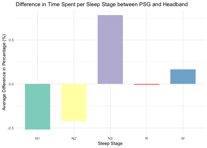

Calculate mean differences and confidence intervals for each sleep stage - Bias

# Calculate mean differences and confidence intervals for each sleep stage
mean_diff_results <- merged_data %>%
  group_by(Sleep_Stage) %>%
  summarise(
    Mean_Difference = mean(Percentage_PSG - Percentage_Headband, na.rm = TRUE),
    SD_Difference = sd(Percentage_PSG - Percentage_Headband, na.rm = TRUE),
    Count = n(),
    SE_Difference = SD_Difference / sqrt(Count),
    CI_Lower = Mean_Difference - qt(0.975, Count - 1) * SE_Difference,  # 95% CI
    CI_Upper = Mean_Difference + qt(0.975, Count - 1) * SE_Difference,
    .groups = 'drop'
  )
# Plot the mean difference with error bars
library(ggplot2)

ggplot(mean_diff_results, aes(x = Sleep_Stage, y = Mean_Difference)) +
  geom_bar(stat = "identity", fill = "lightblue", color = "black") +
  geom_errorbar(aes(ymin = CI_Lower, ymax = CI_Upper), width = 0.2, color = "darkblue") +
  geom_hline(yintercept = 0, linetype = "dashed", color = "red") +  # Line at zero for reference
  labs(title = "Mean Difference in Time Spent in Each Sleep Stage",
       x = "Sleep Stage",
       y = "Mean Difference (PSG - Headband) [%]") +
  theme_minimal()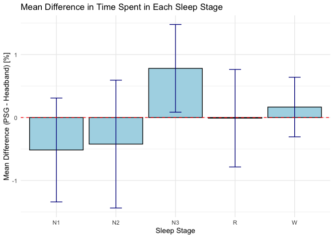

Bland-Altman Statistics

# List of unique sleep stages
sleep_stages <- unique(merged_data$Sleep_Stage)

# Initialize an empty list to store results
ba_results <- list()

# Loop through each sleep stage and calculate Bland-Altman statistics
for (stage in sleep_stages) {
  stage_data <- merged_data %>% filter(Sleep_Stage == stage)
  ba_stats <- blandr.statistics(stage_data$Percentage_PSG, stage_data$Percentage_Headband)
  
  # Append the Bland-Altman statistics object to the list with the stage name
  ba_results[[stage]] <- ba_stats
}

# Print the results for each sleep stage
for (stage in names(ba_results)) {
  cat("\n\nResults for Sleep Stage:", stage, "\n")
  print(ba_results[[stage]])
}

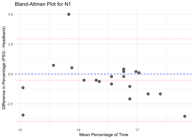
Results for Sleep Stage: N1 
Bland-Altman Statistics
=======================
t = -1.3072, df = 19, p-value = 0.2067
alternative hypothesis: true bias is not equal to 0

=======================
Number of comparisons:  20 
Maximum value for average measures:  17.8125 
Minimum value for average measures:  15.05208 
Maximum value for difference in measures:  5 
Minimum value for difference in measures:  -3.541667 

Bias:  -0.515625 
Standard deviation of bias:  1.76404 

Standard error of bias:  0.3944513 
Standard error for limits of agreement:  0.6856898 

Bias:  -0.515625 
Bias- upper 95% CI:  0.309971 
Bias- lower 95% CI:  -1.341221 

Upper limit of agreement:  2.941893 
Upper LOA- upper 95% CI:  4.377058 
Upper LOA- lower 95% CI:  1.506728 

Lower limit of agreement:  -3.973143 
Lower LOA- upper 95% CI:  -2.537978 
Lower LOA- lower 95% CI:  -5.408308 

=======================
Derived measures:  
Mean of differences/means:  -3.040415 
Point estimate of bias as proportion of lowest average:  -3.425606 
Point estimate of bias as proportion of highest average -2.894737 
Spread of data between lower and upper LoAs:  6.915036 
Bias as proportion of LoA spread:  -7.456577 

=======================
Bias: 
 -0.515625  ( -1.341221  to  0.309971 ) 
ULoA: 
 2.941893  ( 1.506728  to  4.377058 ) 
LLoA: 
 -3.973143  ( -5.408308  to  -2.537978 ) 



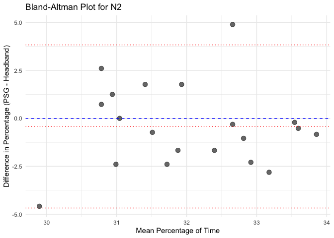
Results for Sleep Stage: N2 
Bland-Altman Statistics
=======================
t = -0.86936, df = 19, p-value = 0.3955
alternative hypothesis: true bias is not equal to 0

=======================
Number of comparisons:  20 
Maximum value for average measures:  33.85417 
Minimum value for average measures:  29.89583 
Maximum value for difference in measures:  4.895833 
Minimum value for difference in measures:  -4.583333 

Bias:  -0.421875 
Standard deviation of bias:  2.170194 

Standard error of bias:  0.4852702 
Standard error for limits of agreement:  0.8435639 

Bias:  -0.421875 
Bias- upper 95% CI:  0.5938073 
Bias- lower 95% CI:  -1.437557 

Upper limit of agreement:  3.831706 
Upper LOA- upper 95% CI:  5.597306 
Upper LOA- lower 95% CI:  2.066107 

Lower limit of agreement:  -4.675456 
Lower LOA- upper 95% CI:  -2.909857 
Lower LOA- lower 95% CI:  -6.441056 

=======================
Derived measures:  
Mean of differences/means:  -1.323016 
Point estimate of bias as proportion of lowest average:  -1.41115 
Point estimate of bias as proportion of highest average -1.246154 
Spread of data between lower and upper LoAs:  8.507162 
Bias as proportion of LoA spread:  -4.959057 

=======================
Bias: 
 -0.421875  ( -1.437557  to  0.5938073 ) 
ULoA: 
 3.831706  ( 2.066107  to  5.597306 ) 
LLoA: 
 -4.675456  ( -6.441056  to  -2.909857 ) 



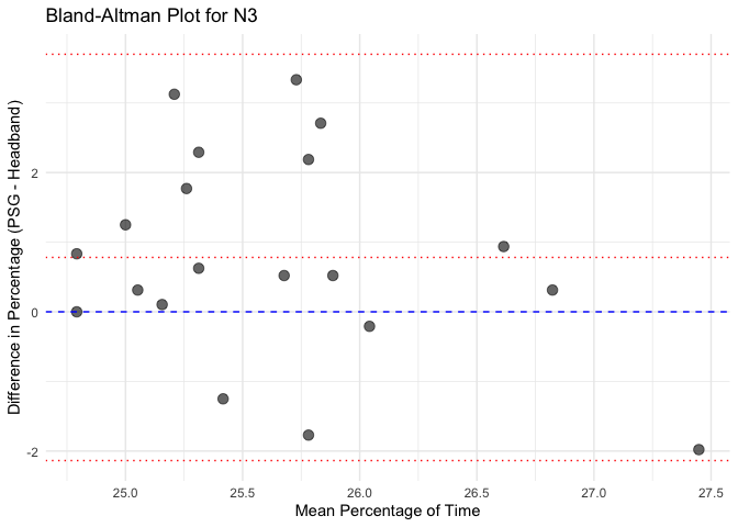
Results for Sleep Stage: N3 
Bland-Altman Statistics
=======================
t = 2.3468, df = 19, p-value = 0.02993
alternative hypothesis: true bias is not equal to 0

=======================
Number of comparisons:  20 
Maximum value for average measures:  27.44792 
Minimum value for average measures:  24.79167 
Maximum value for difference in measures:  3.333333 
Minimum value for difference in measures:  -1.979167 

Bias:  0.78125 
Standard deviation of bias:  1.488757 

Standard error of bias:  0.3328962 
Standard error for limits of agreement:  0.5786862 

Bias:  0.78125 
Bias- upper 95% CI:  1.47801 
Bias- lower 95% CI:  0.08449032 

Upper limit of agreement:  3.699214 
Upper LOA- upper 95% CI:  4.910418 
Upper LOA- lower 95% CI:  2.488009 

Lower limit of agreement:  -2.136714 
Lower LOA- upper 95% CI:  -0.9255094 
Lower LOA- lower 95% CI:  -3.347918 

=======================
Derived measures:  
Mean of differences/means:  3.090366 
Point estimate of bias as proportion of lowest average:  3.151261 
Point estimate of bias as proportion of highest average 2.8463 
Spread of data between lower and upper LoAs:  5.835927 
Bias as proportion of LoA spread:  13.3869 

=======================
Bias: 
 0.78125  ( 0.08449032  to  1.47801 ) 
ULoA: 
 3.699214  ( 2.488009  to  4.910418 ) 
LLoA: 
 -2.136714  ( -3.347918  to  -0.9255094 ) 



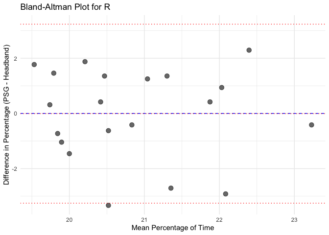
Results for Sleep Stage: R 
Bland-Altman Statistics
=======================
t = -0.028155, df = 19, p-value = 0.9778
alternative hypothesis: true bias is not equal to 0

=======================
Number of comparisons:  20 
Maximum value for average measures:  23.22917 
Minimum value for average measures:  19.53125 
Maximum value for difference in measures:  2.291667 
Minimum value for difference in measures:  -3.333333 

Bias:  -0.01041667 
Standard deviation of bias:  1.654596 

Standard error of bias:  0.3699789 
Standard error for limits of agreement:  0.6431485 

Bias:  -0.01041667 
Bias- upper 95% CI:  0.763958 
Bias- lower 95% CI:  -0.7847913 

Upper limit of agreement:  3.232591 
Upper LOA- upper 95% CI:  4.578716 
Upper LOA- lower 95% CI:  1.886466 

Lower limit of agreement:  -3.253424 
Lower LOA- upper 95% CI:  -1.907299 
Lower LOA- lower 95% CI:  -4.59955 

=======================
Derived measures:  
Mean of differences/means:  -0.0266 
Point estimate of bias as proportion of lowest average:  -0.05333333 
Point estimate of bias as proportion of highest average -0.04484305 
Spread of data between lower and upper LoAs:  6.486016 
Bias as proportion of LoA spread:  -0.1606019 

=======================
Bias: 
 -0.01041667  ( -0.7847913  to  0.763958 ) 
ULoA: 
 3.232591  ( 1.886466  to  4.578716 ) 
LLoA: 
 -3.253424  ( -4.59955  to  -1.907299 ) 



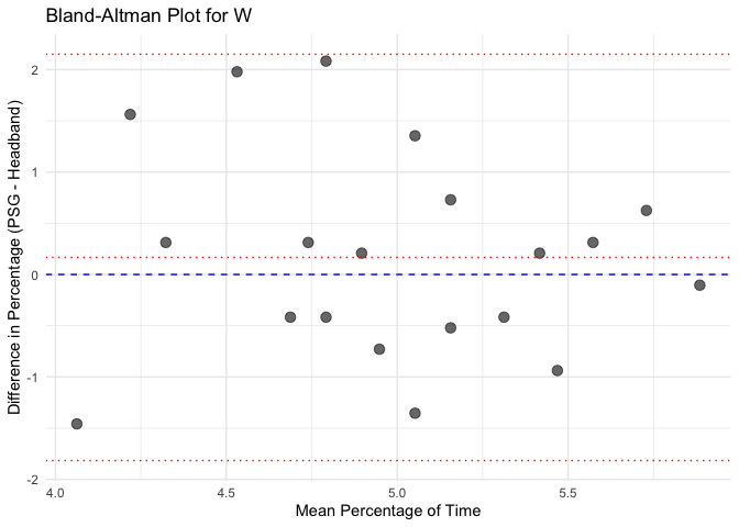
Results for Sleep Stage: W 
Bland-Altman Statistics
=======================
t = 0.73662, df = 19, p-value = 0.4703
alternative hypothesis: true bias is not equal to 0

=======================
Number of comparisons:  20 
Maximum value for average measures:  5.885417 
Minimum value for average measures:  4.0625 
Maximum value for difference in measures:  2.083333 
Minimum value for difference in measures:  -1.458333 

Bias:  0.1666667 
Standard deviation of bias:  1.011854 

Standard error of bias:  0.2262575 
Standard error for limits of agreement:  0.393312 

Bias:  0.1666667 
Bias- upper 95% CI:  0.640229 
Bias- lower 95% CI:  -0.3068956 

Upper limit of agreement:  2.149901 
Upper LOA- upper 95% CI:  2.973112 
Upper LOA- lower 95% CI:  1.326689 

Lower limit of agreement:  -1.816567 
Lower LOA- upper 95% CI:  -0.9933558 
Lower LOA- lower 95% CI:  -2.639779 

=======================
Derived measures:  
Mean of differences/means:  3.584975 
Point estimate of bias as proportion of lowest average:  4.102564 
Point estimate of bias as proportion of highest average 2.831858 
Spread of data between lower and upper LoAs:  3.966468 
Bias as proportion of LoA spread:  4.201891 

=======================
Bias: 
 0.1666667  ( -0.3068956  to  0.640229 ) 
ULoA: 
 2.149901  ( 1.326689  to  2.973112 ) 
LLoA: 
 -1.816567  ( -2.639779  to  -0.9933558 )

# List of unique sleep stages
sleep_stages <- unique(merged_data$Sleep_Stage)

# Initialize an empty list to store results
ba_results <- list()

# Loop through each sleep stage and calculate Bland-Altman statistics
for (stage in sleep_stages) {
  stage_data <- merged_data %>% filter(Sleep_Stage == stage)
  
  # Calculate Bland-Altman statistics
  ba_stats <- blandr.statistics(stage_data$Percentage_PSG, stage_data$Percentage_Headband)
  
  # Append the Bland-Altman statistics object to the list with the stage name
  ba_results[[stage]] <- ba_stats
  
  # Generate the Bland-Altman plot using blandr.draw
  plot_title <- paste('Bland-Altman plot for', stage)  # Concatenate the plot title properly
  ba_plot <- blandr.draw(stage_data$Percentage_PSG, stage_data$Percentage_Headband, 
                         plotTitle = plot_title, ciDisplay = TRUE, ciShading = TRUE)
  
  # Print each plot
  print(ba_plot)
}

Warning: Use of `plot.data$x.axis` is discouraged.
ℹ Use `x.axis` instead.

Warning: Use of `plot.data$y.axis` is discouraged.
ℹ Use `y.axis` instead.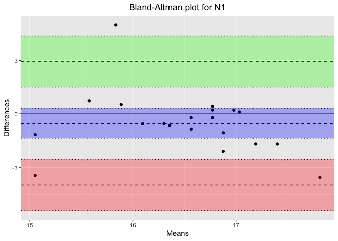

Warning: Use of `plot.data$x.axis` is discouraged.
ℹ Use `x.axis` instead.
Use of `plot.data$y.axis` is discouraged.
ℹ Use `y.axis` instead.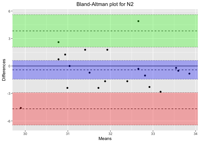

Warning: Use of `plot.data$x.axis` is discouraged.
ℹ Use `x.axis` instead.
Use of `plot.data$y.axis` is discouraged.
ℹ Use `y.axis` instead.

Warning: Use of `plot.data$x.axis` is discouraged.
ℹ Use `x.axis` instead.
Use of `plot.data$y.axis` is discouraged.
ℹ Use `y.axis` instead.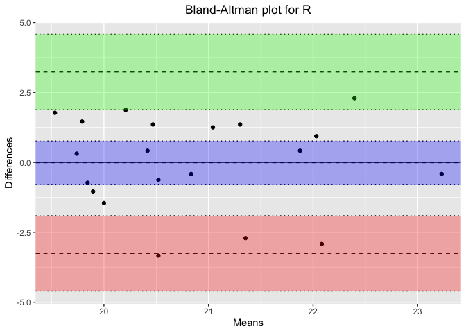

Warning: Use of `plot.data$x.axis` is discouraged.
ℹ Use `x.axis` instead.
Use of `plot.data$y.axis` is discouraged.
ℹ Use `y.axis` instead.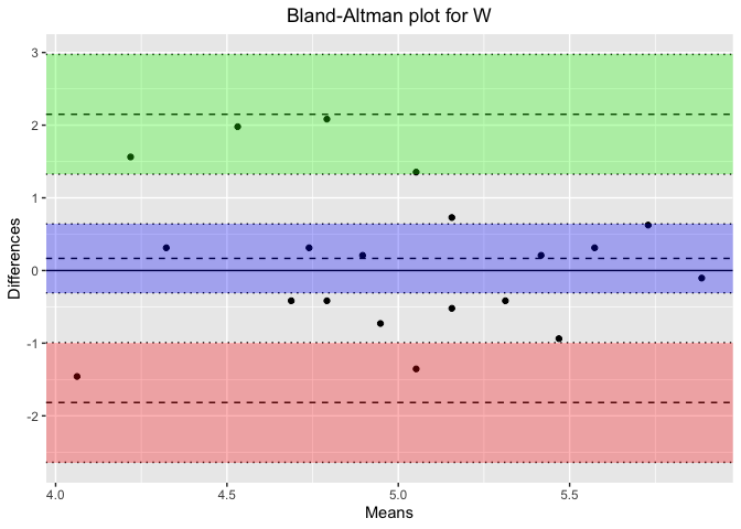

Bland-Altman plots (basic plots, w/o the blandr package)

# Calculate mean and difference for each sleep stage
bland_altman_data <- merged_data %>%
  mutate(Mean = (Percentage_PSG + Percentage_Headband) / 2,
         Difference = Percentage_PSG - Percentage_Headband)

# Create separate Bland-Altman plots for each sleep stage
unique_stages <- unique(bland_altman_data$Sleep_Stage)

# Loop through each sleep stage and create a Bland-Altman plot
for(stage in unique_stages) {
  stage_data <- bland_altman_data %>% filter(Sleep_Stage == stage)
  
  p <- ggplot(stage_data, aes(x = Mean, y = Difference)) +
    geom_point(size = 3, alpha = 0.6) +
    geom_hline(yintercept = 0, linetype = "dashed", color = "blue") +
    geom_hline(aes(yintercept = mean(Difference)), linetype = "dotted", color = "red") +
    geom_hline(aes(yintercept = mean(Difference) + 1.96 * sd(Difference)), linetype = "dotted", color = "red") +
    geom_hline(aes(yintercept = mean(Difference) - 1.96 * sd(Difference)), linetype = "dotted", color = "red") +
    labs(title = paste("Bland-Altman Plot for", stage),
         x = "Mean Percentage of Time",
         y = "Difference in Percentage (PSG - Headband)") +
    theme_minimal()
  
  # Print each plot
  print(p)
}

Calculate Pearson correlation for each sleep stage and each instrument

# Calculate Pearson correlation for each sleep stage
correlation_results <- merged_data %>%
  group_by(Sleep_Stage) %>%
  summarise(Pearson_Correlation = cor(Percentage_PSG, Percentage_Headband, use = "complete.obs"), .groups = 'drop')

# Display the correlation results
# Display the correlation results in a table with a caption and a light blue background
kable(correlation_results, caption = "Pearson Correlation for Each Sleep Stage", digits = 3) %>%
  kable_styling(bootstrap_options = c("striped", "hover")) %>%
  row_spec(0, background = "lightblue")

Pearson Correlation for Each Sleep Stage
Sleep_Stage	Pearson_Correlation
N1	-0.192
N2	0.023
N3	-0.085
R	0.217
W	-0.026

Calculate Cohen’s Kappa for each sleep stage

# Merge PSG and Headband data by Subject_ID and Epoch to align epochs
merged_epochs <- PSG %>%
  select(Subject_ID, Epoch, Sleep_Stage_PSG = Sleep_Stage) %>%
  inner_join(Headband %>% select(Subject_ID, Epoch, Sleep_Stage_Headband = Sleep_Stage),
             by = c("Subject_ID", "Epoch"))

# Calculate Cohen's Kappa for each sleep stage
kappa_results <- lapply(sleep_stages, function(stage) {
  stage_data <- merged_epochs %>%
    filter(Sleep_Stage_PSG == stage | Sleep_Stage_Headband == stage) %>%
    mutate(Sleep_Stage_PSG = ifelse(Sleep_Stage_PSG == stage, 1, 0),
           Sleep_Stage_Headband = ifelse(Sleep_Stage_Headband == stage, 1, 0))
  
  # Calculate Cohen's Kappa for the current stage
  kappa_value <- kappa2(stage_data[, c("Sleep_Stage_PSG", "Sleep_Stage_Headband")], 
                        weight = "unweighted")$value
  
  data.frame(Sleep_Stage = stage, Cohen_Kappa = kappa_value)
})

# Combine results into a single data frame
kappa_results <- do.call(rbind, kappa_results)

# Display the Cohen's Kappa results
kable(kappa_results, caption = "Cohen's Kappa for Each Sleep Stage", digits = 3) %>%
  kable_styling(bootstrap_options = c("striped", "hover")) %>%
  row_spec(0, background = "lightblue")

Cohen's Kappa for Each Sleep Stage
Sleep_Stage	Cohen_Kappa
N1	-0.814
N2	-0.657
N3	-0.590
R	-0.762
W	-0.956

Calculate Intraclass Correlation Coefficient (ICC) for each sleep stage

# Calculate ICC for each sleep stage by using the percentage of time spent in each stage
icc_results <- lapply(sleep_stages, function(stage) {
  stage_data <- merged_data %>%
    filter(Sleep_Stage == stage) %>%
    select(Percentage_PSG, Percentage_Headband)
  
  # Calculate ICC (2,1) for absolute agreement
  icc_value <- icc(stage_data, model = "twoway", type = "agreement", unit = "single")$value
  
  data.frame(Sleep_Stage = stage, ICC = icc_value)
})

# Combine results into a single data frame
icc_results <- do.call(rbind, icc_results)

# Display the ICC results
kable(icc_results, caption = "Intraclass Correlation Coefficient (ICC) for Each Sleep Stage", digits = 3) %>%
  kable_styling(bootstrap_options = c("striped", "hover")) %>%
  row_spec(0, background = "lightblue")

Intraclass Correlation Coefficient (ICC) for Each Sleep Stage
Sleep_Stage	ICC
N1	-0.180
N2	0.023
N3	-0.065
R	0.226
W	-0.026

Calculate Mean Absolute Percentage Error (MAPE) for each sleep stage

mape_results <- merged_data %>%
  mutate(APE = ((Percentage_PSG - Percentage_Headband) / Percentage_PSG) * 100) %>%
  group_by(Sleep_Stage) %>%
  summarise(MAPE = mean(APE, na.rm = TRUE), .groups = 'drop')

mape_results <- mape_results %>%
  mutate(MAPE = paste0(round(MAPE, 2), "%"))

kable(mape_results, caption = "Mean Absolute Percentage Error (MAPE) for Each Sleep Stage", digits = 3) %>%
  kable_styling(bootstrap_options = c("striped", "hover")) %>%
  row_spec(0, background = "lightblue")

Mean Absolute Percentage Error (MAPE) for Each Sleep Stage
Sleep_Stage	MAPE
N1	-3.65%
N2	-1.56%
N3	2.89%
R	-0.33%
W	1.42%

Calculate Concordance Correlation Coefficient (CCC) for each sleep stage

library(DescTools)

Attaching package: 'DescTools'

The following objects are masked from 'package:caret':

    MAE, RMSE

# Calculate CCC for each sleep stage
ccc_results <- lapply(sleep_stages, function(stage) {
  stage_data <- merged_data %>%
    filter(Sleep_Stage == stage) %>%
    select(Percentage_PSG, Percentage_Headband)
  
  ccc_value <- CCC(stage_data$Percentage_PSG, stage_data$Percentage_Headband)$rho.c
  
  data.frame(Sleep_Stage = stage, CCC = ccc_value)
})

# Combine results into a single data frame
ccc_results <- do.call(rbind, ccc_results)

# Display the CCC results
kable(ccc_results, caption = "Concordance Correlation Coefficient (CCC) for Each Sleep Stage") %>%
  kable_styling(bootstrap_options = c("striped", "hover")) %>%
  row_spec(0, background = "lightblue")

Concordance Correlation Coefficient (CCC) for Each Sleep Stage
Sleep_Stage	CCC.est	CCC.lwr.ci	CCC.upr.ci
N1	-0.1693247	-0.5219840	0.2327739
N2	0.0217664	-0.3993760	0.4353233
N3	-0.0617404	-0.3779477	0.2673661
R	0.2169865	-0.2361479	0.5926064
W	-0.0249000	-0.4385490	0.3974549

Calculate Sensitivity for each sleep stage

# Calculate classification metrics for each sleep stage
sensitivity_results <- merged_epochs %>%
  mutate(Agree = (Sleep_Stage_PSG == Sleep_Stage_Headband)) %>%
  group_by(Sleep_Stage_PSG) %>%
  summarise(Sensitivity = mean(Agree), .groups = 'drop')

kable(sensitivity_results, caption = "Sensitivity for Each Sleep Stage") %>%
  kable_styling(bootstrap_options = c("striped", "hover")) %>%
  row_spec(0, background = "lightblue")

Sensitivity for Each Sleep Stage
Sleep_Stage_PSG	Sensitivity
N1	0.1887035
N2	0.3449574
N3	0.4030806
R	0.2380714
W	0.0431211

Compare the confusion matrix between PSG (ground truth) and Headband

confusion_results <- merged_epochs %>%
  mutate(Sleep_Stage_PSG = factor(Sleep_Stage_PSG, levels = sleep_stages),
         Sleep_Stage_Headband = factor(Sleep_Stage_Headband, levels = sleep_stages))

# Generate the confusion matrix
conf_matrix <- confusionMatrix(confusion_results$Sleep_Stage_Headband, confusion_results$Sleep_Stage_PSG)

# Convert confusion matrix table to a data frame for manipulation
conf_matrix_df <- as.data.frame(conf_matrix$table)
colnames(conf_matrix_df) <- c("True_Sleep_Stage", "Predicted_Sleep_Stage", "Frequency")

# Calculate percentages for each row in the confusion matrix
conf_matrix_df <- conf_matrix_df %>%
  group_by(True_Sleep_Stage) %>%
  mutate(Percentage = Frequency / sum(Frequency) * 100)  # Calculate percentages

# Display overall statistics and per-class performance metrics
conf_matrix$overall

      Accuracy          Kappa  AccuracyLower  AccuracyUpper   AccuracyNull 
    0.29713542     0.07340406     0.29067635     0.30365597     0.31812500 
AccuracyPValue  McnemarPValue 
    1.00000000     0.34012087

conf_matrix$byClass

          Sensitivity Specificity Pos Pred Value Neg Pred Value  Precision
Class: N1  0.18870347   0.8366700     0.18289269      0.8418517 0.18289269
Class: N2  0.34495743   0.6882065     0.34044272      0.6924910 0.34044272
Class: N3  0.40308062   0.8004366     0.41554960      0.7920702 0.41554960
Class: R   0.23807145   0.7991709     0.23795256      0.7992761 0.23795256
Class: W   0.04312115   0.9506200     0.04458599      0.9489539 0.04458599
              Recall         F1 Prevalence Detection Rate Detection Prevalence
Class: N1 0.18870347 0.18575265 0.16229167     0.03062500            0.1674479
Class: N2 0.34495743 0.34268521 0.31812500     0.10973958            0.3223437
Class: N3 0.40308062 0.40922015 0.26036458     0.10494792            0.2525521
Class: R  0.23807145 0.23801199 0.20848958     0.04963542            0.2085937
Class: W  0.04312115 0.04384134 0.05072917     0.00218750            0.0490625
          Balanced Accuracy
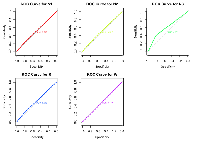
Class: N1         0.5126867
Class: N2         0.5165820
Class: N3         0.6017586
Class: R          0.5186212
Class: W          0.4968706

# Plot the confusion matrix with counts and percentages
ggplot(conf_matrix_df, aes(x = True_Sleep_Stage, y = Predicted_Sleep_Stage, fill = Frequency)) +
  geom_tile() +
  geom_text(aes(label = paste(Frequency, "\n(", round(Percentage, 1), "%)", sep = "")), 
            color = "white", size = 5) +
  scale_fill_gradient(low = "lightblue", high = "blue") +
  labs(title = "Confusion Matrix for PSG (Ground Truth) vs Headband",
       x = "True Sleep Stage (PSG)",
       y = "Predicted Sleep Stage (Headband)") +
  theme_minimal()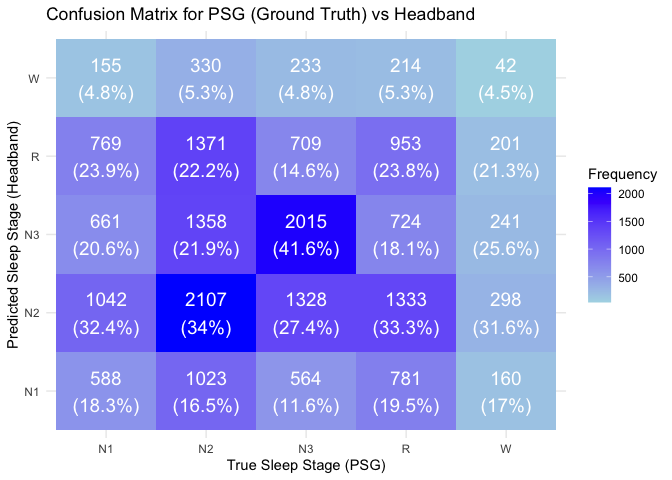

ROC Curves for each sleep stage

# Prepare data for ROC analysis
roc_data <- merged_epochs %>%
  mutate(Sleep_Stage_PSG = factor(Sleep_Stage_PSG, levels = sleep_stages),
         Sleep_Stage_Headband = factor(Sleep_Stage_Headband, levels = sleep_stages))

# Create a list to hold ROC objects for each sleep stage
roc_list <- list()

# Loop through each sleep stage to compute ROC
for(stage in sleep_stages) {
  # Create binary outcomes for the true sleep stage
  roc_data$True_Class <- ifelse(roc_data$Sleep_Stage_PSG == stage, 1, 0)
  roc_data$Predicted_Prob <- as.numeric(roc_data$Sleep_Stage_Headband == stage)  # Assuming you want to predict each stage
  
  # Calculate ROC curve
  roc_curve <- roc(roc_data$True_Class, roc_data$Predicted_Prob, 
                   levels = c(0, 1), direction = "<")
  
  # Store the ROC object in the list
  roc_list[[stage]] <- roc_curve
}


# Plot ROC curves for each sleep stage
par(mfrow=c(2, 3))  # Adjust layout to fit all plots (change as needed)
for(stage in sleep_stages) {
  plot(roc_list[[stage]], 
       col = rainbow(length(sleep_stages))[which(sleep_stages == stage)], 
       main = paste("ROC Curve for", stage), 
       print.auc = TRUE)  # Print AUC on the plot
}